The Phillips curve represents the relationship between the rate of
inflation and the
unemployment rate. Although he had precursors, A. W. H. Phillips's study of wage inflation and unemployment in the United Kingdom from 1861 to 1957 is a milestone in the development of macroeconomics. Phillips found a consistent inverse relationship: when unemployment was high, wages increased slowly; when unemployment was low, wages rose rapidly.
Phillips conjectured that the lower the unemployment rate, the tighter the labor market and, therefore, the faster firms must raise wages to attract scarce labor. At higher rates of unemployment, the pressure abated. Phillips's "curve" represented the average relationship between unemployment and wage behavior over the business cycle. It showed the rate of wage inflation that would result if a particular level of unemployment persisted for some time.
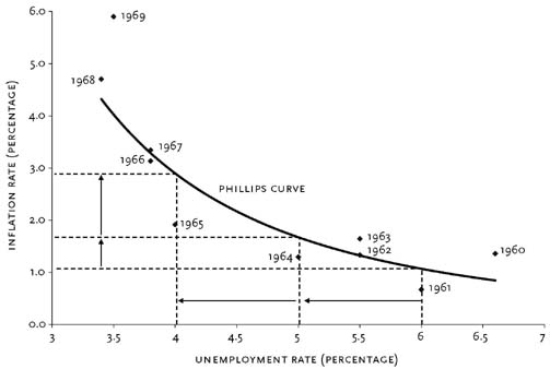
Economists soon estimated Phillips curves for most developed economies. Most related general price inflation, rather than wage inflation, to unemployment. Of course, the prices a company charges are closely connected to the wages it pays. Figure 1 shows a typical Phillips curve fitted to data for the United States from 1961 to 1969. The close fit between the estimated curve and the data encouraged many economists, following the lead of Paul Samuelson and Robert Solow, to treat the Phillips curve as a sort of menu of policy options. For example, with an unemployment rate of 6 percent, the government might stimulate the economy to lower unemployment to 5 percent. Figure 1 indicates that the cost, in terms of higher inflation, would be a little more than half a percentage point. But if the government initially faced lower rates of unemployment, the costs would be considerably higher: a reduction in unemployment from 5 to 4 percent would imply more than twice as big an increase in the rate of inflation—about one and a quarter percentage points.
At the height of the Phillips curve's popularity as a guide to policy, Edmund Phelps and Milton Friedman independently challenged its theoretical underpinnings. They argued that well-informed, rational employers and workers would pay attention only to real wages—the inflation-adjusted purchasing power of money wages. In their view, real wages would adjust to make the supply of labor equal to the demandfor labor, and the unemployment rate would then stand at a level uniquely associated with that real wage—the "natural rate" of unemployment.
Both Friedman and Phelps argued that the government could not permanently trade higher inflation for lower unemployment. Imagine that unemployment is at the natural rate. The real wage is constant: workers who expect a given rate of price inflation insist that their wages increase at the same rate to prevent the erosion of their purchasing power. Now, imagine that the government uses expansionarymonetary or fiscal policy in an attempt to lower unemployment below its natural rate. The resulting increase in demand encourages firms to raise their prices faster than workers had anticipated. With higher revenues, firms are willing to employ more workers at the old wage rates and even to raise those rates somewhat. For a short time, workers suffer from what economists call money illusion: they see that their money wages have risen and willingly supply more labor. Thus, the unemployment rate falls. They do not realize right away that their purchasing power has fallen because prices have risen more rapidly than they expected. But, over time, as workers come to anticipate higher rates of price inflation, they supply less labor and insist on increases in wages that keep up with inflation. The real wage is restored to its old level, and the unemployment rate returns to the natural rate. But the price inflation and wage inflation brought on by expansionary policies continue at the new, higher rates.
Friedman's and Phelps's analyses provide a distinction between the "short-run" and "long-run" Phillips curves. So long as the average rate of inflation remains fairly constant, as it did in the 1960s, inflation and unemployment will be inversely related. But if the average rate of inflation changes, as it will when policymakers persistently try to push unemployment below the natural rate, after a period of adjustment, unemployment will return to the natural rate. That is, once workers' expectations of price inflation have had time to adjust, the natural rate of unemployment is compatible with any rate of inflation. The long-run Phillips curve could be shown on Figure 1 as a vertical line above the natural rate. The original curve would then apply only to brief, transitional periods and would shift with any persistent change in the average rate of inflation. These long-run and short-run relations can be combined in a single "expectations-augmented" Phillips curve. The more quickly workers' expectations of price inflation adapt to changes in the actual rate of inflation, the more quickly unemployment will return to the natural rate, and the less successful the government will be in reducing unemployment through monetary and fiscal policies.
The 1970s provided striking confirmation of Friedman's and Phelps's fundamental point. Contrary to the original Phillips curve, when the average inflation rate rose from about 2.5 percent in the 1960s to about 7 percent in the 1970s, the unemployment rate not only did not fall, it actually rose from about 4 percent to above 6 percent.
Most economists now accept a central tenet of both Friedman's and Phelps's analyses: there is some rate of unemployment that, if maintained, would be compatible with a stable rate of inflation. Many, however, call this the "nonaccelerating inflation rate of unemployment" (NAIRU) because, unlike the term "natural rate," NAIRU does not suggest that an unemployment rate is socially optimal, unchanging, or impervious to policy.
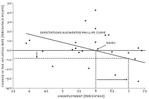
A policymaker might wish to place a value on NAIRU. To obtain a simple estimate, Figure 2 plots changes in the rate of inflation (i.e., the acceleration of prices) against the unemployment rate from 1976 to 2002. The expectations-augmented Phillips curve is the straight line that best fits the points on the graph (the regression line). It summarizes the rough inverse relationship. According to the regression line, NAIRU (i.e., the rate of unemployment for which the change in the rate of inflation is zero) is about 6 percent. The slope of the Phillips curve indicates the speed of price adjustment. Imagine that the economy is at NAIRU with an inflation rate of 3 percent and that the government would like to reduce the inflation rate to zero. Figure 2 suggests that contractionary monetary and fiscal policies that drove the average rate of unemployment up to about 7 percent (i.e., one point above NAIRU) would be associated with a reduction in inflation of about one percentage point per year. Thus, if the government's policies caused the unemployment rate to stay at about 7 percent, the 3 percent inflation rate would, on average, be reduced one point each year—falling to zero in about three years.
Using similar, but more refined, methods, the Congressional Budget Office estimated (Figure 3) that NAIRU was about 5.3 percent in 1950, that it rose steadily until peaking in 1978 at about 6.3 percent, and that it then fell steadily to about 5.2 by the end of the century. Clearly, NAIRU is not constant. It varies with changes in so-called real factors affecting the supply of and demand for labor such as demographics, technology, union power, the structure oftaxation, and relative prices (e.g., oil prices). NAIRU should not vary with monetary and fiscal policies, which affect aggregate demand without altering these real factors.
The expectations-augmented Phillips curve is a fundamental element of almost every macroeconomic forecasting model now used by government and business. It is accepted by most otherwise diverse schools of macroeconomic thought. Early new classical theories assumed that prices adjusted freely and that expectations were formed rationally—that is, without systematic error. These assumptions imply that the Phillips curve in Figure 2 should be very steep and that deviations from NAIRU should be short-lived (see new classical macroeconomics and rational expectations). While sticking to the rational-expectations hypothesis, even new classical economists now concede that wages and prices are somewhat sticky. Wage and price inertia, resulting in real wages and other relative prices away from their market-clearing levels, explain the large fluctuations in unemployment around NAIRU and slow speed of convergence back to NAIRU.
Some "new Keynesian" and some free-market economists hold that, at best, there is only a weak tendency for an economy to return to NAIRU. They argue that there is no natural rate of unemployment to which the actual rate tends to return. Instead, when actual unemployment rises and remains high for some time, NAIRU also rises. The dependence of NAIRU on actual unemployment is known as the hysteresis hypothesis. One explanation for hysteresis in a heavily unionized economy is that unions directly represent the interests only of those who are currently employed. Unionization, by keeping wages high, undermines the ability of those outside the union to compete for employment. After prolonged layoffs, employed union workers may seek the benefits of higher wages for themselves rather than moderating their wage demands to promote the rehiring of unemployed workers. According to the hysteresis hypothesis, once unemployment becomes high—as it did in Europe in the recessions of the 1970s—it is relatively impervious to monetary and fiscal stimuli, even in the short run. The unemployment rate in France in 1968 was 1.8 percent, and in West Germany, 1.5 percent. In contrast, since 1983, both French and West German unemployment rates have fluctuated between 7 and 11 percent. In 2003, the French rate stood at 8.8 percent and the German rate at 8.4 percent. The hysteresis hypothesis appears to be more relevant to Europe, where unionization is higher and where labor laws create numerous barriers to hiring and firing, than it is to the United States, with its considerably more flexible labor markets. The unemployment rate in the United States was 3.4 percent in 1968. U.S. unemployment peaked in the early 1980s at 10.8 percent and fell back substantially, so that by 2000 it again stood below 4 percent.
Modern macroeconomic models often employ another version of the Phillips curve in which the output gap replaces the unemployment rate as the measure of aggregate demand relative to aggregate supply. The output gap is the difference between the actual level of GDP and the potential (or sustainable) level of aggregate output expressed as a percentage of potential. This formulation explains why, at the end of the 1990s boom when unemployment rates were well below estimates of NAIRU, prices did not accelerate. The reasoning is as follows. Potential output depends not only on labor inputs, but also on plant and equipment and other capital inputs. At the end of the boom, after nearly a decade of rapid investment, firms found themselves with too much capital. The excess capacity raised potential output, widening the output gap and reducing the pressure on prices.
Many articles in the conservative business press criticize the Phillips curve because they believe it both implies that growth causes inflation and repudiates the theory that excess growth of money is inflation's true cause. But it does no such thing. One can believe in the Phillips curve and still understand that increased growth, all other things equal, will reduce inflation. The misplaced criticism of the Phillips curve is ironic since Milton Friedman, one of the coinventors of its expectations-augmented version, is also the foremost defender of the view that "inflation is always, and everywhere, a monetary phenomenon."
The Phillips curve was hailed in the 1960s as providing an account of the inflation process hitherto missing from the conventional macroeconomic model. After four decades, the Phillips curve, as transformed by the natural-rate hypothesis into its expectations-augmented version, remains the key to relating unemployment (of capital as well as labor) to inflation in mainstream macroeconomic analysis.

![\mathit{LCSuff}(S_{1..p}, T_{1..q}) = \begin{cases} \mathit{LCSuff}(S_{1..p-1}, T_{1..q-1}) + 1 & \mathrm{if } \; S[p] = T[q] \\ 0 & \mathrm{otherwise} \end{cases}](http://upload.wikimedia.org/math/5/9/b/59bedec58669e638a84364c93529cb4e.png)